Sys.setenv(LANGUAGE = "en")
library(tidyverse)
library(here)
library(scales)
library(gt)
library(fixest)
library(modelsummary)

source(here::here("R", "theme_cours.R"))
set.seed(2024) # the only random draw of the page: simulated scatterplotsSession 4: Descriptive statistics and regression
Summarise, correlate, regress and test: what do the data say about income and health?
Session objectives
- Describe a variable: mean, median, standard deviation, quantiles, IQR, and why GDP per capita needs logs.
- Build a clean summary table with
gt. - Compute and interpret a correlation, and know what it cannot tell you.
- Estimate and read a simple and a multiple regression (
fixest::feols, robust standard errors,modelsummary). - Recognise why pooling years of a few countries produces misleading statistics.
- Optional / homework: run a two-group t-test and interpret the p-value and the confidence interval.
Prepare your R session
Packages used today: tidyverse, here, scales, gt, fixest, modelsummary. If one is missing: install.packages(c("tidyverse", "here", "scales", "gt", "fixest", "modelsummary")).
Script of this session: download seance-4.R, all the code of this page in one file.
Running question: Growth, health and inequality: what do the data say about developing countries? Today, how are income and life expectancy related across countries?
1. One year, one row per country
≈ 15 min After this section you can build a clean one-row-per-country sample and say how many countries it contains.
Sessions 1 and 2 used three countries. Statistics need many units, so we now use all countries. Each statistical method below assumes that one row = one unit. We therefore work on a cross-section: one year, one row per country.
Which year? Let us check coverage of the variables we need.
wdi <- read_csv(here::here("data", "wdi_panel.csv"), show_col_types = FALSE)

wdi |>
  filter(year %in% c(2000, 2010, 2015, 2019, 2021, 2023)) |>
  group_by(year) |>
  summarise(
    countries       = n(),
    `life exp.`     = sum(!is.na(life_exp)),
    `GDP pc`        = sum(!is.na(gdp_pc_ppp)),
    `both`          = sum(!is.na(life_exp) & !is.na(gdp_pc_ppp)),
    `+ Gini`        = sum(!is.na(life_exp) & !is.na(gdp_pc_ppp) & !is.na(gini)),
    `electricity`   = sum(!is.na(elec_access))
  ) |>
  gt() |>
  tab_header(title = "Number of countries with non-missing data") |>
tab_source_note("Source: World Bank, World Development Indicators (WDI). Countries only (aggregates removed).")| Number of countries with non-missing data | ||||||
| year | countries | life exp. | GDP pc | both | + Gini | electricity |
|---|---|---|---|---|---|---|
| 2000 | 217 | 217 | 192 | 192 | 57 | 211 |
| 2010 | 217 | 217 | 198 | 198 | 86 | 215 |
| 2015 | 217 | 217 | 199 | 199 | 87 | 215 |
| 2019 | 217 | 217 | 199 | 199 | 78 | 215 |
| 2021 | 217 | 217 | 199 | 199 | 81 | 215 |
| 2023 | 217 | 217 | 197 | 197 | 60 | 215 |
| Source: World Bank, World Development Indicators (WDI). Countries only (aggregates removed). | ||||||
We use 2019. It is the last year before COVID-19 (which cut life expectancy in 2020-21 and distorts both income and health), and coverage is already at its maximum for GDP per capita and life expectancy. (Sessions 5 and 6 use 2022 instead: they show recent values, and 2022 is the latest year with good coverage.) The Gini index is the weak point: it is only measured in some countries each year.
Check extremes first. The lowest life expectancy in 2019 is the Central African Republic (CAF) at 31.5 years. Before deciding anything, look at the whole series of that country:
wdi |> filter(iso3c == "CAF") |> select(year, life_exp) |> print(n = Inf)# A tibble: 24 × 2
year life_exp
<dbl> <dbl>
1 2000 46.6
2 2001 46.7
3 2002 46.8
4 2003 47.3
5 2004 47.7
6 2005 48.2
7 2006 48.7
8 2007 49.3
9 2008 49.9
10 2009 14.7
11 2010 46.9
12 2011 50.1
13 2012 51.3
14 2013 49.5
15 2014 40.3
16 2015 51.9
17 2016 51.0
18 2017 45.2
19 2018 52.3
20 2019 31.5
21 2020 50.6
22 2021 40.3
23 2022 18.8
24 2023 57.4The series jumps around: 49.9 in 2008 then 14.7 in 2009, 52.3 in 2018 then 31.5 in 2019, 18.8 in 2022 then 57.4 in 2023. Falls of 20 to 35 years followed by an immediate rebound are data artefacts, not findings, and they recur in several years: in this WDI release, no year of the CAF life-expectancy series can be trusted. We never edit the raw file: we exclude the whole CAF series explicitly and say so, and we will do the same in Sessions 5 and 6. CAF therefore leaves the 2019 sample, so N below counts one country fewer.
# CAF life expectancy is unreliable in this WDI release (14.7 in 2009, 18.8 in 2022): exclude every year
wdi <- wdi |> mutate(life_exp = if_else(iso3c == "CAF", NA_real_, life_exp))
cs <- wdi |>
filter(year == 2019, !is.na(life_exp), !is.na(gdp_pc_ppp)) |>
mutate(
income = factor(income, levels = c("Low income", "Lower middle income",
"Upper middle income", "High income")),
log_gdp_pc = log(gdp_pc_ppp)
)
n_cs <- nrow(cs)
n_cs[1] 198Our working sample has 198 countries. Always report N.
ImportantKey idea
Every method in this session assumes one row = one unit. Here the unit is a country in 2019. Before any statistic, know what one row is and how many rows you have.
2. Describing one variable
Centre and spread
≈ 40 min, including Exercise 4.1 After this section you can summarise a variable with the right statistic and explain why GDP per capita is analysed in logs.
The main summaries of a variable \(x_1, \dots, x_N\):
- mean \(\bar{x} = \frac{1}{N}\sum_i x_i\): sensitive to extreme values;
- median: the middle value, robust to extremes;
- standard deviation \(s = \sqrt{\frac{1}{N-1}\sum_i (x_i - \bar{x})^2}\): typical distance to the mean;
- quantiles: the value below which a given share of observations fall; the IQR is the 75th minus the 25th percentile.
mean(cs$life_exp)[1] 72.93089median(cs$life_exp)[1] 73.842sd(cs$life_exp)[1] 7.453676quantile(cs$life_exp, probs = c(0.1, 0.25, 0.5, 0.75, 0.9)) 10% 25% 50% 75% 90%
62.17430 67.04850 73.84200 78.46375 82.60891 IQR(cs$life_exp)[1] 11.41525Standard deviation: the typical distance between a country and the average country. Small \(s\): values cluster around the mean. Large \(s\): they are spread out. It is in the units of the variable (years for life expectancy), so two standard deviations are only comparable for the same variable.
summary() gives the main ones at once:
summary(cs$life_exp) Min. 1st Qu. Median Mean 3rd Qu. Max.
52.99 67.05 73.84 72.93 78.46 85.26 summary(cs$gdp_pc_ppp) Min. 1st Qu. Median Mean 3rd Qu. Max.
1055 6417 16895 26480 38265 133454 Look at GDP per capita: the mean ($26,480) is well above the median ($16,895). A few rich countries pull the mean up. The distribution is right-skewed.
Preview: ggplot is taught in Session 5 and gt tables are only a formatting step. For now, copy the patterns and focus on the statistics.
Show the chart code (taught in Session 5)
mm <- tibble(
  statistic = c("Mean", "Median"),
  value     = c(mean(cs$gdp_pc_ppp), median(cs$gdp_pc_ppp))
)

ggplot(cs, aes(gdp_pc_ppp)) +
  geom_histogram(bins = 30, fill = "grey80", colour = "white") +
  geom_vline(data = mm, aes(xintercept = value, colour = statistic), linewidth = 1.1) +
  scale_colour_manual(values = c(Mean = pal_cours[["accent"]], Median = pal_cours[["principal"]]),
                      labels = c(Mean = "Mean", Median = "Median")) +
  scale_x_continuous(labels = label_dollar()) +
  labs(
    title = "A few rich countries drag the mean above the median",
    x = "GDP per capita (2021 PPP $)", y = "Number of countries", colour = NULL,
    caption = paste0("Source: World Bank, World Development Indicators (WDI), 2019. N = ", n_cs, " countries.")
  ) +
  theme(legend.position = "top")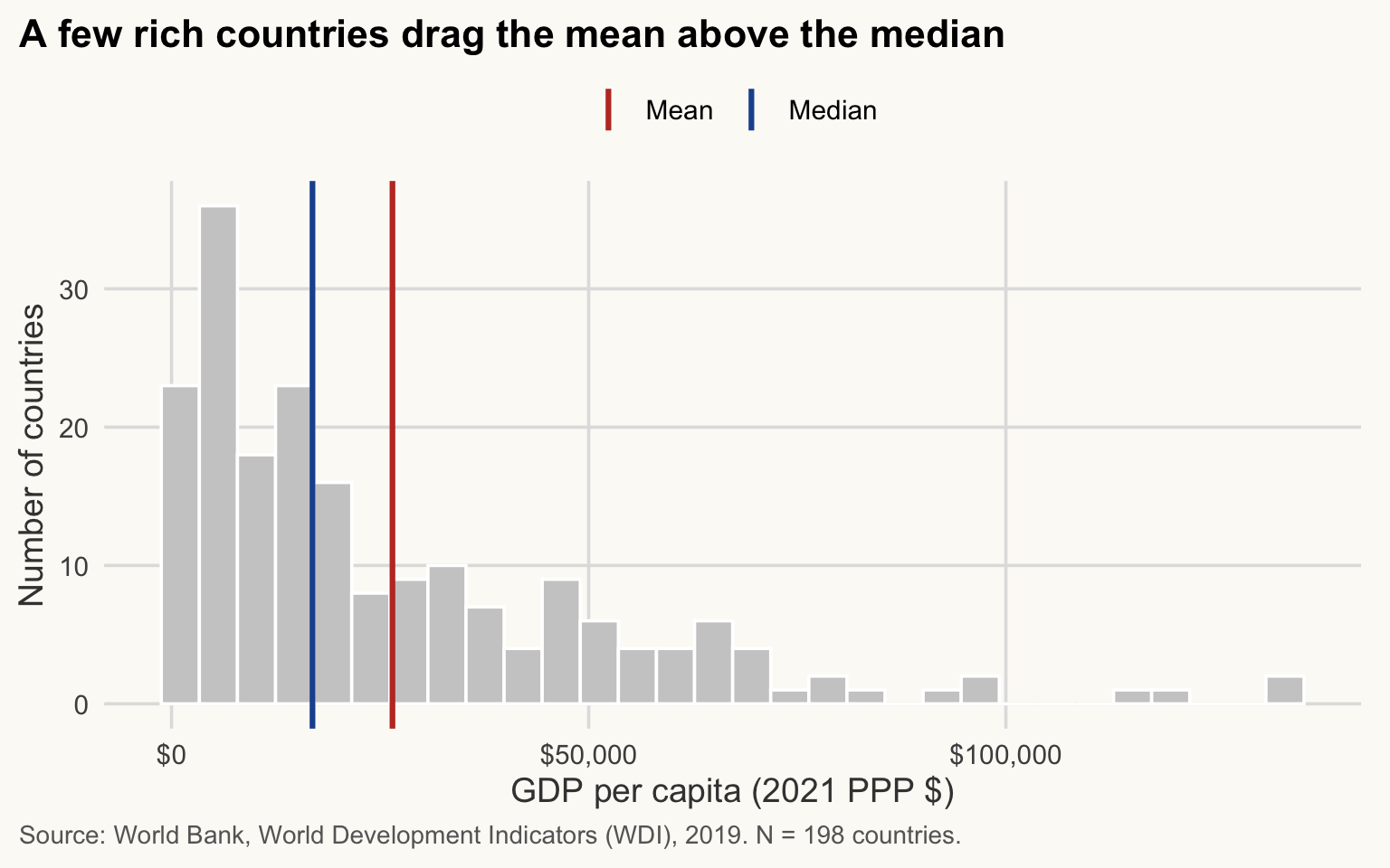
NoteHow to read this chart
- Each bar counts the countries in a range of GDP per capita; most of the mass is on the left.
- The blue line (median) splits the countries in two equal halves. The red line (mean) sits to its right because the few very rich countries in the tail pull it up.
- The further apart the two lines, the more skewed the variable. For a symmetric variable they would coincide.
cs |>
  select(gdp_pc_ppp, log_gdp_pc) |>
  pivot_longer(everything(), names_to = "variable", values_to = "value") |>
  # factor(): fix the panel order and give each variable a readable label
  mutate(variable = factor(variable,
                           levels = c("gdp_pc_ppp", "log_gdp_pc"),
                           labels = c("GDP per capita (2021 PPP $)", "Log of GDP per capita"))) |>
  ggplot(aes(value)) +
  geom_histogram(bins = 25, fill = pal_cours[["principal"]], colour = "white") +
  facet_wrap(~ variable, scales = "free_x") +
  scale_x_continuous(labels = label_number(big.mark = ",")) +
  labs(
    title = "Most countries are poor; a few are very rich",
    x = NULL, y = "Number of countries",
    caption = paste0("Source: World Bank, World Development Indicators (WDI), 2019. N = ", n_cs, " countries.")
  )
NoteHow to read this chart
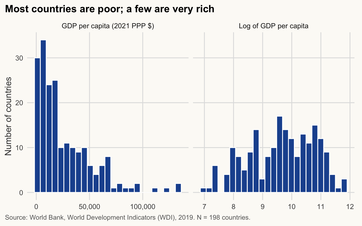
- Left panel: levels. Almost all countries are squeezed into the first bars and a long tail runs to the right.
- Right panel: logs. The same countries are now spread out in a roughly symmetric bell shape.
- Same data, different scale: the log does not change the ranking of countries, only how distances between them are measured.
Why logs? A log turns multiplicative differences into additive ones: going from $1,000 to $2,000 is the same step as from $20,000 to $40,000 (+100%). Income gaps between countries are better thought of in percentages than in dollars. The log is also what makes the relationship with life expectancy close to linear (Section 4).
ImportantKey idea
When a variable is right-skewed, the mean describes the few rich countries as much as the typical one. Report the median, and analyse income in logs.
By group
group_by() + summarise() (Session 3) gives the statistics by group. The groups are the income group (current World Bank classification): the variable income holds each country’s group today, applied to every year, so a country that has since moved up appears in its current group even in 2019.
by_inc <- cs |>
  group_by(income) |>
  summarise(
    N          = n(),
    mean_le    = mean(life_exp),
    median_le  = median(life_exp),
    sd_le      = sd(life_exp),
    iqr_le     = IQR(life_exp)
  )
by_inc
# A tibble: 4 × 6
income N mean_le median_le sd_le iqr_le
<fct> <int> <dbl> <dbl> <dbl> <dbl>
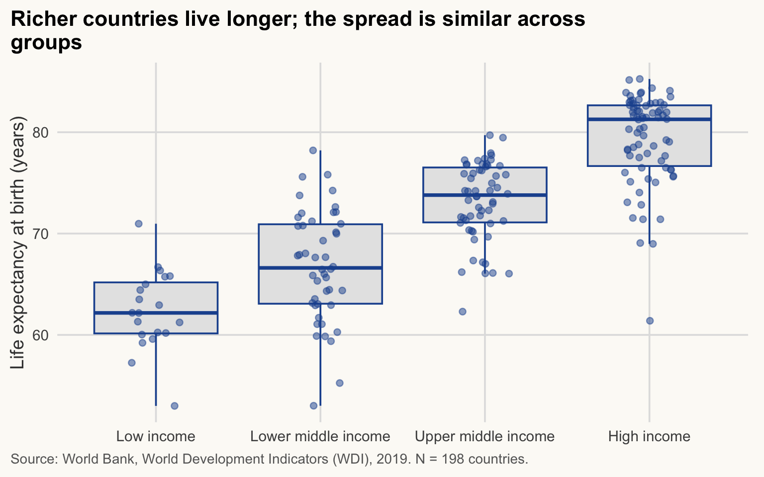
1 Low income 20 62.4 62.2 3.93 5.04
2 Lower middle income 46 66.8 66.6 5.44 7.84
3 Upper middle income 58 73.2 73.8 3.87 5.42
4 High income 74 79.4 81.3 4.45 5.99ggplot(cs, aes(income, life_exp)) +
geom_boxplot(fill = "grey90", colour = pal_cours[["principal"]], outlier.shape = NA) +
geom_jitter(width = 0.15, alpha = 0.5, colour = pal_cours[["principal"]]) +
labs(
title = str_wrap("Richer countries live longer; the spread is similar across groups", 60),
x = NULL, y = "Life expectancy at birth (years)",
caption = str_wrap(paste0("Source: World Bank, World Development Indicators (WDI), 2019. N = ", n_cs, " countries."), 95)
)
NoteHow to read this chart
- Each box covers the middle 50% of countries of a group (25th to 75th percentile); the thick line inside is the median; each dot is one country.
- Compare the heights of the boxes: they rise from low to high income, so richer groups live longer.
- Compare the sizes of the boxes: they are similar. The widest is the lower-middle-income group (IQR of 7.8 years in the table above, against 5.0 to 6.0 for the other groups). Being richer does not make a group more homogeneous.
A tidy summary table
A table for a paper has formatted numbers, an N column and a source note. gt builds it from a data frame.
cs |>
  group_by(region) |>
  summarise(
    N               = n(),
    gdp_mean        = mean(gdp_pc_ppp),
    gdp_median      = median(gdp_pc_ppp),
    le_mean         = mean(life_exp),
    le_sd           = sd(life_exp)
  ) |>
  arrange(desc(le_mean)) |>
  gt() |>
  cols_label(
    region     = "Region",
    N          = "N",
    gdp_mean   = "Mean",
    gdp_median = "Median",
    le_mean    = "Mean",
    le_sd      = "Std. dev."
  ) |>
  tab_spanner("GDP per capita (2021 PPP $)", c(gdp_mean, gdp_median)) |>
  tab_spanner("Life expectancy (years)", c(le_mean, le_sd)) |>
  fmt_currency(c(gdp_mean, gdp_median), decimals = 0) |>
  fmt_number(c(le_mean, le_sd), decimals = 1) |>
  tab_header(title = "Income and life expectancy by region, 2019") |>
tab_source_note("Source: World Bank, World Development Indicators (WDI). One observation per country; N = number of countries. Regions are World Bank categories.")| Income and life expectancy by region, 2019 | |||||
| Region | N |
GDP per capita (2021 PPP $)
|
Life expectancy (years)
|
||
|---|---|---|---|---|---|
| Mean | Median | Mean | Std. dev. | ||
| North America | 3 | $74,076 | $69,121 | 80.7 | 1.7 |
| Europe & Central Asia | 53 | $42,973 | $38,182 | 78.4 | 4.3 |
| Middle East, North Africa, Afghanistan & Pakistan | 22 | $29,106 | $14,968 | 75.7 | 5.9 |
| Latin America & Caribbean | 38 | $23,822 | $21,578 | 74.5 | 3.7 |
| South Asia | 6 | $11,699 | $11,129 | 73.5 | 3.9 |
| East Asia & Pacific | 31 | $26,963 | $11,629 | 72.8 | 7.0 |
| Sub-Saharan Africa | 45 | $6,482 | $3,557 | 63.3 | 4.7 |
| Source: World Bank, World Development Indicators (WDI). One observation per country; N = number of countries. Regions are World Bank categories. | |||||
TipExercise 4.1
Produce, by income group, a gt table with N, the mean and the median of elec_access (access to electricity, % of population) in 2019. Drop countries with missing elec_access and say how many. What do mean and median tell you in the low-income group?
NoteShow solution
elec <- cs |> filter(!is.na(elec_access))
nrow(cs) - nrow(elec)   # countries dropped
[1] 1elec |>
group_by(income) |>
summarise(N = n(), mean = mean(elec_access), median = median(elec_access)) |>
gt() |>
fmt_number(c(mean, median), decimals = 1) |>
tab_header(title = "Access to electricity (% of population), 2019") |>
tab_source_note("Source: World Bank, World Development Indicators (WDI). N = number of countries with data.")| Access to electricity (% of population), 2019 | |||
| income | N | mean | median |
|---|---|---|---|
| Low income | 20 | 38.1 | 30.9 |
| Lower middle income | 46 | 73.6 | 76.0 |
| Upper middle income | 57 | 96.5 | 99.7 |
| High income | 74 | 99.8 | 100.0 |
| Source: World Bank, World Development Indicators (WDI). N = number of countries with data. | |||
low <- elec |> filter(income == "Low income")
c(mean = mean(low$elec_access), median = median(low$elec_access))
mean median
38.08 30.95 In the low-income group the median (30.9%) is below the mean (38.1%): a few countries with high access pull the mean up, so the distribution is right-skewed. Access is very unequal even among poor countries.
3. Correlation
≈ 30 min, including Exercise 4.2 After this section you can compute a correlation, test it, and explain what it does and does not tell you.
The correlation coefficient measures the strength of the linear association between two variables:
\[ r_{XY} = \frac{\operatorname{cov}(X, Y)}{\sigma_X \, \sigma_Y}, \qquad -1 \le r_{XY} \le 1 . \]
It is the covariance rescaled by the two standard deviations, so it does not depend on units. \(r = 1\): perfect upward line; \(r = -1\): perfect downward line; \(r = 0\): no linear association.
Correlation (\(r\)): a number between -1 and 1 that says how closely two variables move along a straight line, and in which direction. Rule of thumb: |r| below 0.3 is weak, above 0.7 is strong. It says nothing about which variable influences the other.
n_sim <- 200
x <- rnorm(n_sim)
make_y <- function(r, x) r * x + sqrt(1 - r^2) * rnorm(length(x))

x_u <- runif(n_sim, -2, 2)
sim <- bind_rows(
  tibble(x = x,   y = make_y(0.9, x),  panel = "Strong positive"),
  tibble(x = x,   y = make_y(0, x),    panel = "No relationship"),
  tibble(x = x,   y = make_y(-0.9, x), panel = "Strong negative"),
  tibble(x = x_u, y = x_u^2,           panel = "Strong but non-linear")
) |>
  group_by(panel) |>
  mutate(r = cor(x, y)) |>
  ungroup() |>
  # fct_inorder(): keep the panels in their order of appearance, not alphabetical
  mutate(panel = fct_inorder(paste0(panel, " (r = ", sprintf("%.2f", r), ")")))

ggplot(sim, aes(x, y)) +
  geom_point(alpha = 0.6, colour = pal_cours[["principal"]]) +
  facet_wrap(~ panel, scales = "free") +
  labs(
    title = str_wrap("r measures linear association, not whether two variables are related", 60),
    x = "X", y = "Y",
    caption = str_wrap("Source: simulated data.", 95)
  )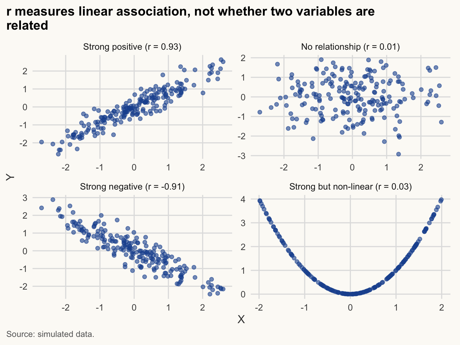
The last panel is the key lesson: \(Y = X^2\) is a deterministic relationship, yet \(r \approx 0\). Always plot before you correlate.
NoteHow to read this chart
- Each panel is a cloud of 200 points; the tighter the cloud around a line, the closer |r| is to 1.
- Panel 2: a shapeless cloud, r near 0. Panel 4: a perfect U-shape, yet r near 0, because the line it would need is not straight.
- A number like r hides the shape of the data. The plot shows it.
Now the real data: income and life expectancy.
r_lin <- cor(cs$gdp_pc_ppp, cs$life_exp, use = "complete.obs")
r_log <- cor(cs$log_gdp_pc, cs$life_exp, use = "complete.obs")
c(levels = r_lin, logs = r_log)
levels logs
0.7394593 0.8564695 The correlation with GDP per capita in levels is 0.74; with the log it is 0.86. The relationship is much closer to a straight line in logs, so the log is the right scale.
ct <- cor.test(cs$log_gdp_pc, cs$life_exp)
ct
    Pearson's product-moment correlation

data:  cs$log_gdp_pc and cs$life_exp
t = 23.229, df = 196, p-value < 2.2e-16
alternative hypothesis: true correlation is not equal to 0
95 percent confidence interval:
 0.8142747 0.8896611
sample estimates:
      cor
0.8564695
cor.test() tests \(H_0: \rho = 0\). Here \(r\) = 0.86, with a 95% confidence interval of [0.81, 0.89] and N = 198. The p-value is below \(10^{-15}\): we reject zero correlation. But a tiny p-value does not say the correlation is causal or important; it says it is unlikely to be pure sampling noise.
p-value: if there were truly no relationship in the population, how often would we see a correlation (or gap, or coefficient) at least this large just by chance? A small p-value means “hard to blame on chance”. It does not say the effect is large, important or causal.
WarningCommon mistake
Correlation is not causation. Income and life expectancy move together (r close to 0.86 in logs), but the correlation alone cannot say whether income raises health, health raises income, or something else (institutions, education, climate) drives both. Before writing “X leads to Y”, ask: could Y cause X? Could a third variable cause both?
TipExercise 4.2
Compute the correlation between elec_access and life_exp in the 2019 cross-section (use = "complete.obs"), run cor.test(), and draw the scatterplot. Is a straight line a reasonable summary?
NoteShow solution
cor(cs$elec_access, cs$life_exp, use = "complete.obs")[1] 0.7504866cor.test(cs$elec_access, cs$life_exp)
    Pearson's product-moment correlation

data:  cs$elec_access and cs$life_exp
t = 15.857, df = 195, p-value < 2.2e-16
alternative hypothesis: true correlation is not equal to 0
95 percent confidence interval:
 0.6822713 0.8057475
sample estimates:
      cor
0.7504866
cs |>
filter(!is.na(elec_access)) |>
ggplot(aes(elec_access, life_exp)) +
geom_point(alpha = 0.6, colour = pal_cours[["principal"]]) +
labs(
title = str_wrap("Life expectancy rises with electricity access, but the link bends", 60),
x = "Access to electricity (% of population)",
y = "Life expectancy at birth (years)",
caption = str_wrap("Source: World Bank, World Development Indicators (WDI), 2019.", 95)
)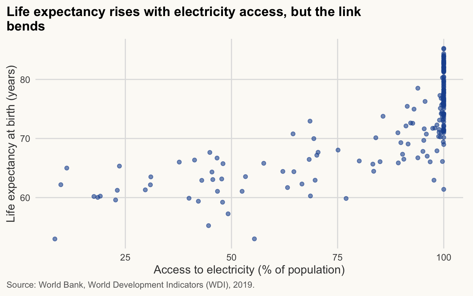
Most countries are near 100% access; the relationship is steep only at low access, so a single straight line is a rough summary. This is a feature of the data (a ceiling), not an error.
ImportantKey idea
A correlation is a one-number summary of a straight-line pattern. Plot first, check the scale (logs), then correlate, and never read it as cause and effect.
4. Simple regression
≈ 40 min, including Exercise 4.3 After this section you can fit a simple regression, read its slope in the units of the data, and explain what a residual is.
Correlation is symmetric and unit-free. A regression gives a slope in the units of the data:
\[ \text{life\_exp}_i = \alpha + \beta \, \ln(\text{GDP pc}_i) + \varepsilon_i . \]
OLS chooses \(\alpha, \beta\) to minimise the sum of squared residuals \(\sum_i \hat{\varepsilon}_i^2\).
NoteIn plain words
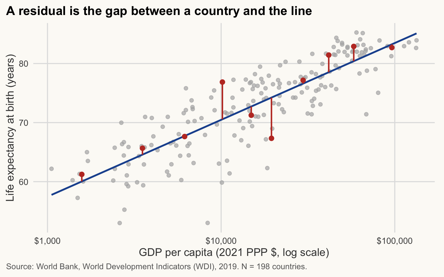
Imagine drawing a straight line through the cloud of countries. For each country, the residual is the vertical gap between the country and the line: how much its real life expectancy differs from what the line predicts. OLS picks the line that makes these gaps, squared and added up, as small as possible.
Three things to know before the code.
-
Formulas. R writes a model as
y ~ x1 + x2: the outcome on the left of~, the explanatory variables on the right, separated by+. The intercept is added automatically. -
lm()vsfeols().lm()is base R and gives the same coefficients. We usefixest::feols()because it handles standard errors more conveniently and extends to the fixed-effects models you will meet later. -
vcov = "hetero"asks for heteroskedasticity-robust standard errors: they stay valid when the spread of the errors differs across countries, which is the usual case. It changes the standard errors, not the coefficients. It does not fix omitted-variable bias or reverse causality: those are problems of the model, not of the standard errors.
Robust standard error: an estimate of how much a coefficient would vary from sample to sample, computed without assuming that the errors have the same spread for every country. It changes the width of the confidence interval and the p-value, never the coefficient itself.
WarningCommon mistake
Using robust standard errors and concluding that the estimate is “causal”. Robust SEs only make the uncertainty more honest. If income and health are both driven by institutions, the coefficient is biased whatever the standard errors are.
m1 <- feols(life_exp ~ log_gdp_pc, data = cs, vcov = "hetero")
summary(m1)
OLS estimation, Dep. Var.: life_exp
Observations: 198
Standard-errors: Heteroskedasticity-robust
Estimate Std. Error t value Pr(>|t|)
(Intercept) 18.44317 2.201431 8.37781 1.0268e-14 ***
log_gdp_pc 5.64837 0.219547 25.72742 < 2.2e-16 ***
---
Signif. codes: 0 '***' 0.001 '**' 0.01 '*' 0.05 '.' 0.1 ' ' 1
RMSE: 3.83784 Adj. R2: 0.732181b1 <- coef(m1)[["log_gdp_pc"]](We created log_gdp_pc beforehand; feols(life_exp ~ log(gdp_pc_ppp)) would give the same result.)
Reading the coefficient (log-level model). \(\hat\beta\) = 5.65 years. Because GDP enters in logs:
- a 1% increase in GDP per capita is associated with \(\hat\beta / 100 \approx\) 0.056 more years of life expectancy;
- a 10% increase is associated with about \(\hat\beta \times \ln(1.1) = \hat\beta \times 0.0953 \approx\) 0.54 years;
- doubling GDP per capita is associated with \(\hat\beta \times \ln 2 \approx\) 3.92 years.
The intercept (18.4) is the predicted life expectancy at \(\ln(\text{GDP pc}) = 0\), i.e. GDP pc of $1: outside the data, so not interpretable.
\(R^2\) is the share of the variance of life expectancy “explained” by the line: here 0.73, which is also \(r^2\) from Section 3. Note the quotation marks: explained means statistically accounted for, not caused.
Show the chart code (taught in Session 5)
cs_fit <- cs |>
  mutate(fitted_le = fitted(m1)) |>
  arrange(gdp_pc_ppp)

# ten countries spread along the income distribution
shown <- cs_fit |> slice(round(seq(5, nrow(cs_fit) - 4, length.out = 10)))

ggplot(cs_fit, aes(gdp_pc_ppp, life_exp)) +
  geom_point(colour = "grey70", alpha = 0.7) +
  geom_line(aes(y = fitted_le), colour = pal_cours[["principal"]], linewidth = 1.1) +
  geom_segment(data = shown, aes(xend = gdp_pc_ppp, yend = fitted_le),
               colour = pal_cours[["accent"]], linewidth = 0.9) +
  geom_point(data = shown, colour = pal_cours[["accent"]], size = 2.5) +
  scale_x_log10(labels = label_dollar()) +
  labs(
    title = "A residual is the gap between a country and the line",
    x = "GDP per capita (2021 PPP $, log scale)",
    y = "Life expectancy at birth (years)",
    caption = paste0("Source: World Bank, World Development Indicators (WDI), 2019. N = ", n_cs, " countries.")
  )
NoteHow to read this chart
- The blue line is the prediction: for a given GDP per capita, the life expectancy the model expects.
- Each red segment is one residual: positive above the line (the country lives longer than predicted), negative below it.
- OLS chooses the line that minimises the sum of the squared lengths of all the gaps, not only the red ones.
ggplot(cs, aes(gdp_pc_ppp, life_exp)) +
  geom_point(alpha = 0.6, colour = pal_cours[["principal"]]) +
  geom_smooth(method = "lm", formula = y ~ x, colour = pal_cours[["accent"]],
              fill = pal_cours[["accent"]], alpha = 0.15) +
  scale_x_log10(labels = label_dollar()) +
  labs(
    title = "Richer countries have longer life expectancy",
    x = "GDP per capita (2021 PPP $, log scale)",
    y = "Life expectancy at birth (years)",
    caption = paste0("Source: World Bank, World Development Indicators (WDI), 2019. N = ", n_cs, " countries.")
  )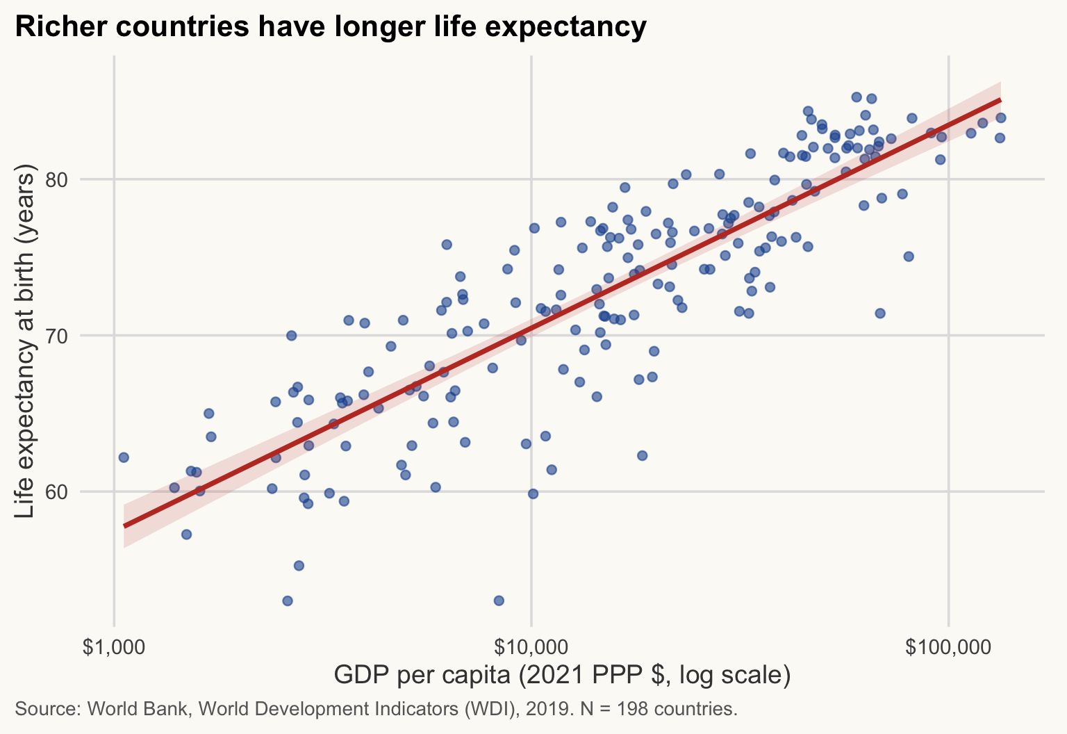
With a log x-axis, the fitted relationship is a straight line, which is exactly the log-level model.
NoteHow to read this chart
- Each dot is a country; the line is the OLS fit and the shaded band its 95% confidence interval.
- The slope of the line is \(\hat\beta\): the gain in years per unit of natural log GDP. The axis ticks are powers of ten, so one tick to the next (a tenfold income difference) is \(\hat\beta \times \ln 10 \approx\) 13 years.
- Dots far from the line are countries much healthier or sicker than their income predicts. The band shows uncertainty about the line, not about each country.
NoteWhy it matters for development economics
The income-health gradient (the “Preston curve”) is a starting point for questions about aid and growth: does raising incomes buy longer lives? This regression cannot answer that, but it shows the size of the gap that any explanation has to account for.
ImportantKey idea
In a log-level regression, the slope \(\hat\beta\) is read per 1% (divide by 100) or per doubling (multiply by 0.69) of income. It is a difference between countries, not what would happen to one country that grows.
TipExercise 4.3
Regress life_exp on elec_access in the 2019 cross-section (feols, robust SEs). Interpret the slope in one sentence (units!), give \(R^2\) and N, and say what you would worry about before reading it as an effect of electrification.
NoteShow solution
m_el <- feols(life_exp ~ elec_access, data = cs, vcov = "hetero")
summary(m_el)
OLS estimation, Dep. Var.: life_exp
Observations: 197
Standard-errors: Heteroskedasticity-robust
Estimate Std. Error t value Pr(>|t|)
(Intercept) 52.607599 1.281582 41.0489 < 2.2e-16 ***
elec_access 0.234818 0.014405 16.3010 < 2.2e-16 ***
---
Signif. codes: 0 '***' 0.001 '**' 0.01 '*' 0.05 '.' 0.1 ' ' 1
RMSE: 4.92181 Adj. R2: 0.56099r2(m_el, "r2") r2
0.5632302 The slope is the difference in life expectancy (years) associated with one more percentage point of the population having electricity access. N is the number of countries with non-missing elec_access. Worries: omitted variables (income, institutions, health spending drive both), reverse causality (healthier, richer societies electrify), and non-linearity (ceiling at 100%).
5. Multiple regression
≈ 40 min, including Exercise 4.4 After this section you can read a multi-model regression table, and explain why changing the sample and changing the specification must not be confused.
Is the income-health relationship just a proxy for something else? Add controls:
\[ \text{life\_exp}_i = \alpha + \beta \ln(\text{GDP pc}_i) + \gamma \, \text{Gini}_i + \delta' \text{Region}_i + \varepsilon_i . \]
First, the cost: the Gini is missing for many countries.
n_gini <- cs |> filter(!is.na(gini)) |> nrow()
tibble(sample = c("All countries", "With Gini"), N = c(n_cs, n_gini))
# A tibble: 2 × 2
sample N
<chr> <int>
1 All countries 198
2 With Gini 78N falls from 198 to 78. Adding the Gini therefore changes two things at once: the specification and the sample. To compare fairly, we also re-estimate the simple model on the sample with Gini.
relevel() sets the reference category of the region dummies: coefficients on the other regions are differences relative to Sub-Saharan Africa.
cs_g <- cs |>
  filter(!is.na(gini)) |>
  mutate(region = relevel(factor(region), ref = "Sub-Saharan Africa"))
cs <- cs |>
  mutate(region = relevel(factor(region), ref = "Sub-Saharan Africa"))

m2 <- feols(life_exp ~ log_gdp_pc,               data = cs_g, vcov = "hetero")
m3 <- feols(life_exp ~ log_gdp_pc + gini,        data = cs_g, vcov = "hetero")
m4 <- feols(life_exp ~ log_gdp_pc + gini + region, data = cs_g, vcov = "hetero")
nice_names <- function(x) {
x |>
str_replace("^log_gdp_pc$", "Log GDP per capita") |>
str_replace("^gini$", "Gini index (0-100)") |>
str_replace("^region", "Region: ") |>
str_replace("^\\(Intercept\\)$", "Constant")
}
modelsummary(
output = "gt", # a gt table: same look as the other tables, no external script
fmt = \(x) nb(x, 3), # decimal mark of the page language
list("(1) All" = m1, "(2) With Gini" = m2, "(3) + Gini" = m3, "(4) + Region" = m4),
coef_rename = nice_names,
stars = c("*" = 0.1, "**" = 0.05, "***" = 0.01),
gof_map = c("nobs", "r.squared"),
title = "Life expectancy, 2019 cross-section (OLS)",
notes = c("Dependent variable: life expectancy at birth (years). Heteroskedasticity-robust standard errors in parentheses.",
"Region reference category: Sub-Saharan Africa.",
"Source: World Bank, World Development Indicators (WDI), 2019. Columns (2)-(4) use only countries with a Gini index.")
)| (1) All | (2) With Gini | (3) + Gini | (4) + Region | |
|---|---|---|---|---|
| Constant | 18.443*** | 23.529*** | 22.586*** | 22.071*** |
| (2.201) | (3.305) | (4.324) | (5.358) | |
| Log GDP per capita | 5.648*** | 5.267*** | 5.311*** | 5.143*** |
| (0.220) | (0.317) | (0.341) | (0.508) | |
| Gini index (0-100) | 0.014 | 0.027 | ||
| (0.047) | (0.066) | |||
| Region: East Asia & Pacific | 1.908 | |||
| (2.089) | ||||
| Region: Europe & Central Asia | 1.750 | |||
| (2.146) | ||||
| Region: Latin America & Caribbean | 1.785 | |||
| (2.179) | ||||
| Region: Middle East, North Africa, Afghanistan & Pakistan | 2.911 | |||
| (2.386) | ||||
| Region: North America | 0.567 | |||
| (2.850) | ||||
| Region: South Asia | 4.869** | |||
| (1.871) | ||||
| Num.Obs. | 198 | 78 | 78 | 78 |
| R2 | 0.734 | 0.771 | 0.771 | 0.788 |
| * p < 0.1, ** p < 0.05, *** p < 0.01 | ||||
| Dependent variable: life expectancy at birth (years). Heteroskedasticity-robust standard errors in parentheses. | ||||
| Region reference category: Sub-Saharan Africa. | ||||
| Source: World Bank, World Development Indicators (WDI), 2019. Columns (2)-(4) use only countries with a Gini index. | ||||
gdp3    <- coef(m3)[["log_gdp_pc"]]
se_gdp3 <- se(m3)[["log_gdp_pc"]]
b <- round(c(coef(m1)[["log_gdp_pc"]], coef(m2)[["log_gdp_pc"]],
             coef(m3)[["log_gdp_pc"]], coef(m4)[["log_gdp_pc"]]), 2)
bg  <- coef(m3)[["gini"]]
bg4 <- coef(m4)[["gini"]]
se3 <- se(m3)[["gini"]]
p3  <- pvalue(m3)[["gini"]]
p4  <- pvalue(m4)[["gini"]]
NoteHow to read this table
Read one row, one column at a time. Take the row “Log GDP per capita” in column (3):
- Coefficient (5.31): the difference in life expectancy, in years, associated with one more unit of log GDP per capita, holding the Gini fixed.
- Standard error (in parentheses, 0.34): the uncertainty on the coefficient. A rough rule: the coefficient is “distinguishable from zero” if it is more than about 2 standard errors away (here 15.6).
- Stars: a shortcut for the p-value (* p < 0.1, ** p < 0.05, *** p < 0.01). More stars mean “harder to blame on chance”, not “bigger effect”.
- R² (bottom): the share of the variance of life expectancy accounted for by the model in that column.
- Num.Obs. (N): the number of countries used. It changes between columns (1) and (2): compare the sample before comparing the estimates.
How to read the four columns together (the table above has all the numbers):
- Columns (1) and (2) give the same kind of estimate on two samples: the GDP coefficient is 5.65 with all countries and 5.27 with the countries that have a Gini (N = 198 vs 78). Sample composition matters.
- Column (3): adding the Gini barely moves the GDP coefficient (5.27 to 5.31). The Gini coefficient is 0.014 (robust SE 0.047, p = 0.76): a 10-point higher Gini goes with about 0.14 years of life expectancy, holding income constant. That is small, and statistically indistinguishable from zero.
- Column (4): with region dummies the GDP coefficient is 5.14 and the Gini coefficient 0.027 (p = 0.68), again small and not significant. The income gradient survives the controls; it is not simply a regional effect.
Show the chart code (taught in Session 5)
modelplot(
  list("(1) All" = m1, "(2) With Gini" = m2, "(3) + Gini" = m3, "(4) + Region" = m4),
  coef_rename = nice_names,
  coef_omit = "Intercept|region"
) +
  geom_vline(xintercept = 0, linetype = "dashed", colour = "grey40") +
  scale_colour_manual(values = unname(c(pal_cours[["gris"]], pal_cours[["principal"]],
                                        pal_regions[["Sub-Saharan Africa"]], pal_cours[["accent"]]))) +
  labs(
    title = "The income gradient is stable; the Gini coefficient is near zero",
    x = "Coefficient (years of life expectancy per unit), 95% CI", y = NULL, colour = NULL,
    caption = "Source: World Bank, World Development Indicators (WDI), 2019. Columns (2)-(4): countries with a Gini index."
  ) +
  theme(legend.position = "bottom")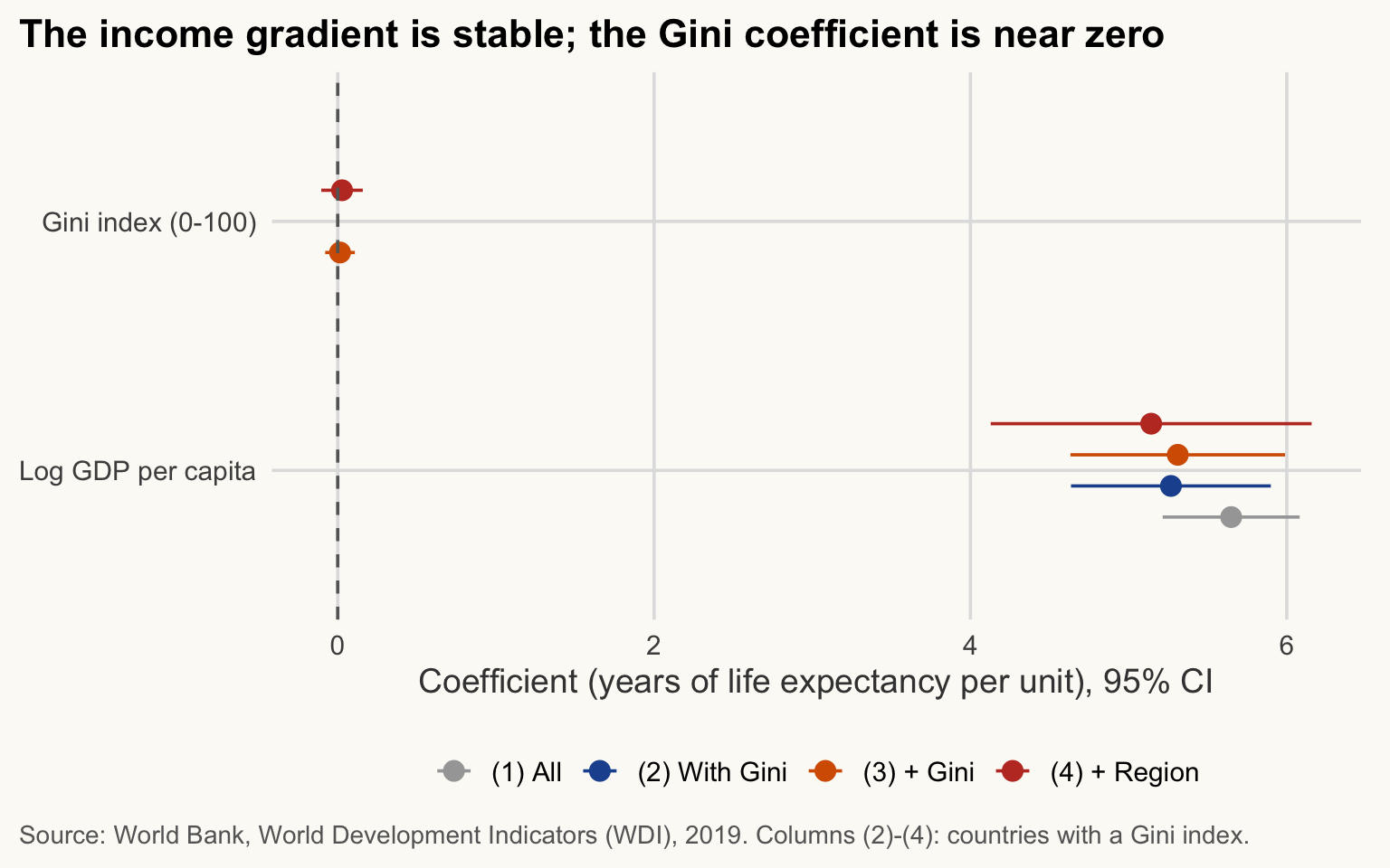
NoteHow to read this chart
- Each dot is a coefficient; the horizontal bar is its 95% confidence interval. The dashed line is zero.
- A bar that does not touch zero (log GDP) is distinguishable from no relationship. A bar that crosses zero (Gini) is not.
- The two variables are on different scales (log points vs Gini points), so compare each bar with zero, not one variable with the other.
Each coefficient is “the difference associated with a one-unit change, holding the other included variables fixed”. These are associations, not causal effects:
- Omitted variables: institutions, health systems, education, climate and conflict affect both income and health.
- Reverse causality: healthier populations are more productive, so health may raise income as well as the opposite.
- Measurement and selection: the Gini is available for a non-random subset of countries, and it mixes two kinds of household surveys: consumption-based (common in low-income countries, India for example) and income-based (most high-income countries). Consumption is less unequally distributed than income, so the same Gini value does not measure the same thing everywhere.
- Not independent draws: neighbouring countries share climate, history and institutions, so observations are correlated within regions. And our 2019 countries are close to the whole population of countries, not a random sample of it, so read p-values as a rough guide to noise, not as exact probabilities.
ImportantKey idea
“Holding the other variables fixed” is a statement about the model, not about the world. A coefficient moves only when you add a variable that is correlated with both the outcome and the variable of interest, and the sample must stay the same for the comparison to be fair.
TipExercise 4.4
Estimate life_exp ~ log_gdp_pc + elec_access on the 2019 cross-section. Does the coefficient on log GDP per capita change compared to Model (1) estimated on the same countries? Why, in words?
NoteShow solution
cs_el  <- cs |> filter(!is.na(elec_access))   # same sample for both models
m1_el  <- feols(life_exp ~ log_gdp_pc,               data = cs_el, vcov = "hetero")
m_ctrl <- feols(life_exp ~ log_gdp_pc + elec_access, data = cs_el, vcov = "hetero")
etable(m1_el, m_ctrl)
m1_el m_ctrl
Dependent Var.: life_exp life_exp
Constant 18.35*** (2.204) 23.41*** (2.212)
log_gdp_pc 5.655*** (0.2198) 4.441*** (0.3156)
elec_access 0.0770*** (0.0186)
_______________ _________________ __________________
S.E. type Heteroskeda.-rob. Heteroskedas.-rob.
Observations 197 197
R2 0.73624 0.76288
Adj. R2 0.73489 0.76044
---
Signif. codes: 0 '***' 0.001 '**' 0.01 '*' 0.05 '.' 0.1 ' ' 1elec_access is missing for 1 country, so Model (1) is first re-estimated on the same 197 countries. On that sample, the income coefficient falls from 5.65 to 4.44 when access is added. Electricity access is itself strongly correlated with income, and also with life expectancy: part of what the income coefficient captured is now attributed to access, so the income coefficient shrinks.
6. Why not pool years?
≈ 10 min After this section you can explain why a panel of a few countries is not a large sample.
WarningPooling years of a few countries does not give independent observations
A common mistake: regress GDP on year, or compare two regions, using 21 years for each of three countries. Two problems:
- Non-independence. The 21 observations of China are the same country, strongly correlated from one year to the next. 63 country-years from 3 countries is not a sample of size 63: observations of the same country are far from independent. Standard errors, t-tests and p-values computed as if they were would be far too optimistic.
- Spurious regression. Any two series that trend upward over time (GDP, population, CO2, the number of smartphones) are strongly correlated, whatever the causal link. A high \(R^2\) between two trending series is the default outcome, not evidence.
A failed join can also silently drop a country (the US in the Session 3 example), so always check N and join keys (anti_join(), Session 3). The fixes used today: a cross-section (one row per country), N reported everywhere, and, for panels, methods designed for them (fixed effects, clustered standard errors), which you will meet in a more advanced course.
7. Optional / homework: hypothesis testing and a model table
≈ 30 min After this section you can test a difference between two groups and say what a p-value does and does not mean.
This section is not needed for the next sessions. Do it at home or if you finish early.
Question: is life expectancy different in Sub-Saharan Africa than elsewhere? One observation per country, one year: the unit of observation is the country, and countries are not strictly independent draws (see Section 5).
cs_t <- cs |>
  mutate(group = if_else(region == "Sub-Saharan Africa", "Sub-Saharan Africa", "Rest of the world"))

cs_t |>
  group_by(group) |>
  summarise(N = n(), mean = mean(life_exp), sd = sd(life_exp))
# A tibble: 2 × 4
group N mean sd
<chr> <int> <dbl> <dbl>
1 Rest of the world 153 75.8 5.46
2 Sub-Saharan Africa 45 63.3 4.72The Welch t-statistic compares two means without assuming equal variances:
\[ t = \frac{\bar{x}_1 - \bar{x}_2}{\sqrt{\dfrac{s_1^2}{n_1} + \dfrac{s_2^2}{n_2}}} . \]
The numerator is the observed gap; the denominator is its standard error. A large \(|t|\) means the gap is large relative to what sampling noise could produce under \(H_0: \mu_1 = \mu_2\).
tt <- t.test(life_exp ~ group, data = cs_t)   # Welch by default
tt
    Welch Two Sample t-test

data:  life_exp by group
t = 15.058, df = 81.75, p-value < 2.2e-16
alternative hypothesis: true difference in means between group Rest of the world and group Sub-Saharan Africa is not equal to 0
95 percent confidence interval:
 10.85315 14.15737
sample estimates:
 mean in group Rest of the world mean in group Sub-Saharan Africa
                        75.77300                         63.26774
gap <- unname(tt$estimate[1] - tt$estimate[2])Reading it. The mean life expectancy is 75.8 years in the rest of the world and 63.3 in Sub-Saharan Africa: a gap of 12.5 years (\(t\) = 15.1, p-value <1e-15). The 95% confidence interval for the gap is [10.9, 14.2] years. In plain words: if we repeatedly drew such samples, intervals built this way would contain the true gap 95% of the time; here the interval is far from zero.
What a p-value is not.
- It is not the probability that \(H_0\) is true. It is the probability of a gap at least this large if \(H_0\) were true.
- It is not the size of the effect: with large samples, trivial gaps get tiny p-values. Look at the gap and the confidence interval.
- “Not significant” is not “no difference”: it may just be low power.
- It says nothing about why the groups differ.
TipExercise 4.5
- Test whether life expectancy differs between high-income countries and all others (2019, one row per country). Report N in each group, the gap, the 95% CI and your interpretation. (b) Build a
modelsummarytable with two models of your choice (for examplelife_exp ~ log_gdp_pcandlife_exp ~ log_gdp_pc + elec_access) with robust SEs, a note defining the stars, and readable coefficient names.
NoteShow solution
# (a) high-income vs the rest
cs_h <- cs |> mutate(group = if_else(income == "High income", "High income", "Other"))
count(cs_h, group)
# A tibble: 2 × 2
group n
<chr> <int>
1 High income 74
2 Other 124t.test(life_exp ~ group, data = cs_h)
    Welch Two Sample t-test

data:  life_exp by group
t = 13.633, df = 188.35, p-value < 2.2e-16
alternative hypothesis: true difference in means between group High income and group Other is not equal to 0
95 percent confidence interval:
  8.795007 11.770882
sample estimates:
mean in group High income       mean in group Other
                 79.37072                  69.08777
# (b) two models in one table
ma <- feols(life_exp ~ log_gdp_pc, data = cs, vcov = "hetero")
mb <- feols(life_exp ~ log_gdp_pc + elec_access, data = cs, vcov = "hetero")
modelsummary(
output = "gt", # a gt table: same look as the other tables, no external script
fmt = \(x) nb(x, 3), # decimal mark of the page language
list("(1)" = ma, "(2)" = mb),
coef_rename = c("log_gdp_pc" = "Log GDP per capita",
"elec_access" = "Electricity access (%)",
"(Intercept)" = "Constant"),
stars = c("*" = 0.1, "**" = 0.05, "***" = 0.01),
gof_map = c("nobs", "r.squared"),
notes = c("Dependent variable: life expectancy (years). Robust standard errors in parentheses.",
"* p < 0.1, ** p < 0.05, *** p < 0.01. Source: World Bank, World Development Indicators (WDI), 2019.")
)| (1) | (2) | |
|---|---|---|
| Constant | 18.443*** | 23.408*** |
| (2.201) | (2.212) | |
| Log GDP per capita | 5.648*** | 4.441*** |
| (0.220) | (0.316) | |
| Electricity access (%) | 0.077*** | |
| (0.019) | ||
| Num.Obs. | 198 | 197 |
| R2 | 0.734 | 0.763 |
| * p < 0.1, ** p < 0.05, *** p < 0.01 | ||
| Dependent variable: life expectancy (years). Robust standard errors in parentheses. | ||
| * p < 0.1, ** p < 0.05, *** p < 0.01. Source: World Bank, World Development Indicators (WDI), 2019. | ||
In (a), the group labelled “High income” is the first in the output only alphabetically; read the two means carefully to get the sign of the gap right.
Key takeaways
- Report N everywhere; know your unit of observation (here: a country in 2019).
- Skewed variables: the mean is pulled by extremes; use the median and logs. GDP per capita is analysed in logs.
- \(r = \operatorname{cov}(X,Y)/(\sigma_X \sigma_Y)\) measures linear association only: plot first.
- In a log-level regression, 1% more GDP per capita goes with \(\beta/100\) more years; a 10% increase with \(\beta \times 0.0953\).
- Adding a variable with missing values changes the sample: compare models on the same sample.
- Regression coefficients are associations; omitted variables and reverse causality prevent a causal reading.
- A p-value is not the probability that \(H_0\) is true, and says nothing about the size of an effect: read the confidence interval.